Thermal Systems Day Two: The Puzzle of MATLAB continues.....

Today, my partner Kirstin and I expanded our simulated behavior from the previous day to an actual thermal system, namely a resistor with a sensor attached to it. The sensor, called a thermistor, would measure the heat dissipated by the resistor, which we could control by altering the energy output of the system.

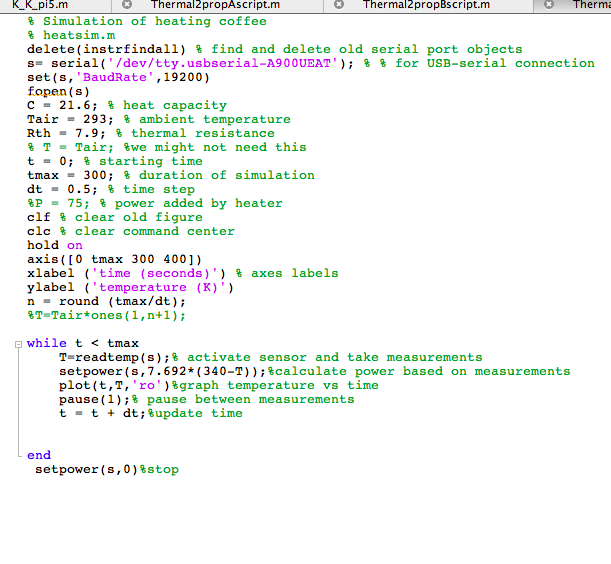
Our first experiment was to determine the physical constants (Rth and C) from our simulated heating experiment in order to conduct our experimental run.

Using:

Rth = (T-Tair)/p

And the knowledge that our maximum power was 6.5 volts.

(354.92 - 303.5)/6.5 = 7.9 T/W

And 

C= p/initial slope of graph

C = 6.5/ [(325.5-312.3)T/(54-10)s) = 21.6 W/(T/s)

Because (Rth)*(C) = ti, the time constant or time in which it would take our system to reach 63.2% of its final asymptotic value, we could check our answers.

(7.9)*(21.6) = 170.64

At this time in seconds, out graph was approximately two thirds the way to its final value, so we knew we were correct.

Our two calculated values were dramatically different from our simulated values in the previous post because of the dramatic change in power. Now, we only had a 6.5 v battery to power our system, so the answer had to adhere to this stipulation. 

Next, we modified our simulated heating program to incorporate these parameters. 

Our simulated heater evenly tapers off and maintains a constant temperature once it reaches the desired temperature. Additionally, the incline is smooth, whereas the experimentally measured incline was rougher. This is probably the result of slightly fluctuating surrounding air temperatures or wind.  However, just line the experimentally measured values, the temperature rises more sharply at the beginning and then gently tapers off to a smaller slope.

Next, Kirsten and I constructed a bang-bang controlled heater that would raised the temperature to the desired value and then try to keep it there. 

Bang-Bang control experimental script

Bang-bang control experimental graph

Unlike our simulated bang-bang control, the experimental graph did not fluctuate evenly on it reached the desired temperature. Instead, it bounced randomly to different values around the desired temperature based on the system was interacting with the air temperature around it. It behaved more like a realistic system should because it is a real system. Next, Kirsten and I implemented Proportional Control to help our system. To do this, we experimented with various proportional gains (.05, .2, and .5). We had to calculate the coefficients each time. To do this, we set up a proportionality ratio:

100 is to 6.5 as (blank) is to .05

Our calculated coefficients were:

.7679 for .05, 3.077 for .2, and 7.692 for .5

Finally, we inserted these values into our coefficients into the script to observe their effects.

.5 Gain

.2 Gain

.05 Gain

Our results were varied, but after ultimately the coefficient of 7.69 proved to be the best option for our realistic system.

Gain of .5, Coefficient 7.69

Gain of .2, Coefficient 3.077

Gain of .05, Coefficient .769

Ultimately, the experimental system never reached its target Temperature of 340 Kelvin. When the proportional gain is small, the system does not add enough power to reach its destination. Even when there is a large difference between the final and initial temperatures, the small coefficient results in a low power setting. Conversely, a large coefficient results in a much larger power setting. When Kp was almost 8, the system did come extremely close to reaching it's goal. 

Graph of Simulated Proportional Control

                              

Unlike our simulation, the experimental graphs never made it to 350 Kelvin, let alone exceed it.

Finally, we constructed our very own PI Controller. A Pi Controller incorporates both integral and proportional control to achieve and maintain a certain temperature. 

Script PI Controller

                              

Script PI Controller and Graphs of Temperature and Power vs Time

After a bit of experimentation, we found that the Ki value from the equation: 

P_desired = Kp*error+Ki*integral_error

Was approximately .5. However, we ended up having to increase our Kp value from 7.69 to 12 in order for the system to eventually reach its destination. The graph shows that, even when we blew on the resistor, thus cooling it, the temperature remained mostly constant while the power fluctuated heavily in order to maintain this constant temperature. Unlike our simulated PI Controller from the previous post, this controller did not fluctuate so dramatically or predictably. More often than not, as evidenced by the above red line on the upper graph, the temperature was constant, even under cooling conditions. 

Simulated PI Controller and Graph